Social Media is the new hype today. Be it Facebook, Instagram, Twitter, other blogs like this one, there are different media sources today to express just about anything. And this easy availability is a data warehouse, just waiting to be picked and analysed.

Data on Twitter for example, is mainly public. Unless explicitly set, all tweets and retweets from anyone with a Twitter account is accessible and readable by anyone in the world, and this provides us with a perfect opportunity.

This blog post, is going to delve into one such aspect. Text Mining using Twitter. I am doing this for the first time as well, so hopefully, this works out as planned.

I will be using RStudio, R3.03 and the freely available twitteR package. Also, 95% of the code will be directly plagiarised from http://www.rdatamining.com/examples/text-mining. Copyright notice and all that.

What is R?

For that, we have Wikipedia.

But in essence, R is a (relatively) new programming language that is fast reaching cult status. It’s extremely powerful, small, and most importantly: open source. That means, everything is free, everything is available, everything is transparent, and most importantly, it allows avid programmers to create their own remarkable packages to be shared online and used by anyone for free.

R is primarily a statistical analysis tool, but is powerful enough that you can do just about anything from basic C adapted code, to text processing, and to more complex statistical analysis.

Installing R is extremely simple. Just Google R3.0.3 and RStudio. Rstudio is an IDE, or an Integrated Development Environment, much like Spyder for Python and Eclipse for Android Development. An IDE makes coding a lot faster, and a lot more efficient. It is in essence, a layer over the primary programming software (in our case R3.0.3) that works as a powerful front end.

Instead of manually typing the code into the R Console or R shell, using RStudio, we get all the perks an IDE offers, like Autocompletion, Documentation, Syntax Correction, Variable Explorers etc. All the small things that make coding so much more enjoyable.

Once you install R3.0.3 and RStudio, RStudio should automatically locate your system’s R software and that’s it, we’re good to go. For a more detailed step by step manual, visit here. (No, I haven’t put a link, it’s actually that easy. But if you really need help, just Google. There are countless blogs and tutorials on how to just install R.)

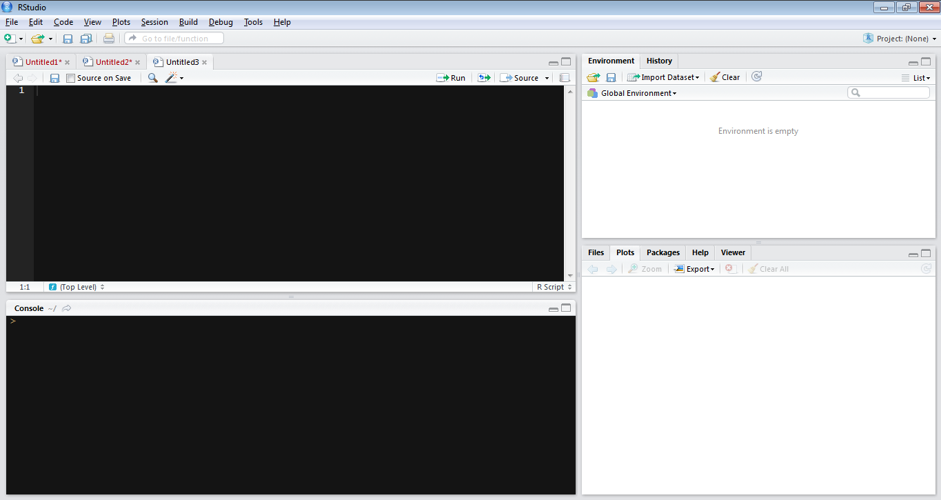
Ok, moving on. Once you run RStudio, you should get an interface like this:  (I’ve customized mine to look dark, it’s generally 2 big white blogs)

First thing to do is to fire up a new R Script (Ctrl+Shift+N for those who appreciate shortcuts) and a text editor panel should appear above your R console. This is where you’ll want to type and run most of your code. Alternatively, you could just enter it line by line into the console, but that gets ugly for longer codes.

We’re not just ready yet, as per new Twitter regulations, anytime you wish to use a third party software, or an API to access the twitter database, you need to register yourself as a Twitter developer. This process takes 2 minutes if you already have a twitter account, or about 5 if you don’t. It’s a one time thing, and is needed if you want to proceed here.

A step by step tutorial for the same can be found here: http://geoffjentry.hexdump.org/twitteR.pdf

But what you really need from that link is just this:

“The first step is to create a Twitter application for yourself. Go to https: //twitter.com/apps/new and log in. After filling in the basic info, go to the “Settings” tab and select ”Read, Write and Access direct messages”. Make sure to click on the save button after doing this. In the “Details” tab, take note of your consumer key and consumer secret”

Ok, that’s done and dusted.

Back to our R script. And now, we get to the part where we actually write code (phew!)

Quick R tips:

1. Highly recommend typing in the editor instead of in the console
2. To run a section of code, select the text in the editor and select RUN, or Ctrl+Enter
3. Ctrl+Space will be your magic potion. Once a variable is run in the console, it gets saved in that R session. So if I have a term This_is_a_sample_variable, all I need to do is type in once in the editor, along with the subsequent value(you’ll understand more a few paragraphs down), and the next time, all I have to do is start typing Th and hit Ctrl+Space, it should automatically populate, or provide a dropdown list of similar words/functions/terms/variables.
4. R is case sensitive, the twitteR package in R has to be spelt that way, and not “twitter”. You’ll get used to it, and another reason why Ctrl+Space is so useful
5. Unlike other generic IDEs with external packages, installing a package in R is hilariously simple. All you need to do is type install.packages(“PackageName”) and run the code. All dependencies, shell paths, everything gets set. Once the package is installed, to activate it for your current session, use library(PackageName) (unlike Python with the pips, easy_installs, PythonPATH and what not.)

<<Wait a minute, a final thing to be done, if you’re using R for the first time, and on Windows. You will need to install an R package called RCurl which is used for certificate sharing. Don’t worry about the meaning, the certificate sharing is just a way of confirming to twitter through R that you are indeed running code to access Twitter, and you’re not a nasty unknown virus hell bent on taking revenge for Ellen’s famous Oscar Selfie. To complete the certification sharing, just copy the following lines into your Rscript:

install.packages(RCurl)

library (RCurl)
download.file(url=”http://curl.haxx.se/ca/cacert.pem&#8221;, destfile=”cacert.pem”)
options(RCurlOptions = list(cainfo = system.file(“CurlSSL”, “cacert.pem”, package = “RCurl”)))

You don’t have to worry about what it means, you’ll never have to debug it. For those of you who don’t really want to understand the code, just feel free to avoid anything mentioned in << >>

The next bit of code you have to enter into your Script window editor is:

install.packages(twitteR)
library(twitteR)

reqURL <-“ https://api.twitter.com/oauth/request_token”
accessURL <- “https://api.twitter.com/oauth/access_token”
authURL <- “https://api.twitter.com/oauth/authorize”
apiKey <- “ENTER YOUR API KEY HERE, WITHIN THESE QUOTATION MARKS”
apiSecret <- “ENTER YOUR API SECRET HERE, WITHIN THESE QUOTATION MARKS”

<<R syntax lesson. In R, the <- operator is similar to the = operator in most languages (in some cases, we can go ahead and just use the = in R itself.) What it does is basically assigns everything after the <- to the variable before the symbol. This makes it easier to just plug in the variable further down instead of repeating all the lines in the end. The above variables are all string variables, which mean they have to be enclosed in quotation marks, and can contain textual data. If numbers are stored within quotation marks, they lose their numeric property. So while

a<-2
b<-3
a+b

should give a result of 5

a<-”2”
b<-“3”
a+b will give an error because we can’t perform arithmetic addition on characters.>>

twitCred <- OAuthFactory$new(consumerKey=apiKey,consumerSecret=apiSecret,requestURL=reqURL,accessURL=accessURL,authURL=authURL)
twitCred$handshake(cainfo = system.file(“CurlSSL”, “cacert.pem”, package = “RCurl”))

This is when you should get a message similar to the one above, this is the second verification stage. Just copy the link mentioned (right from the https://) and paste it in your internet browser. After logging in, you should get a 6-8 digit code, just enter that in the console. You might not be able to see it as you type it in, but that’s ok. Once you’re done, hit enter.

registerTwitterOAuth(twitCred)

If everything worked fine, you should get a TRUE message, otherwise, you’ll need to back track and correct something.

People who know the basics of programming will know the jist of what’s going on here. In essence, we are accessing a function that passes the values which we’ve stored in the variables above, and the function does all the processing at the back end, to make sure we can access tweets without any worries.  The function can be found inbuilt within the twitteR package.

For people who don’t know the basics of programming: We use funny words and special characters to give us twitter data. Abracadabra. 🙂

thetweets<- userTimeline(“ENTER TWITTER USERNAME HERE”, n=ENTER NUMBER OF TWEETS HERE)
n<- length(thetweets)

What we are doing here is assigning another variable (mytweets) to store all the twitter data we are searching for.

I’m an avid football fan, and an Arsenal supporter. Optajoe is a twitter account that gives interesting football statistics. Let’s get into meta mode and try and analyse the analysis of football, shall we?

I want to access the last 100 tweets of optajoe and store them in a variable called thetweets. I also want to store the number of tweets I’m actually able to pull up into a variable n, for which I use another function available in R called length(). When you execute this, you might notice that the value of n might not match with the limit you set. This could be because either that user doesn’t have the number of tweets specified by “n” or that the function is only storing a specific type of tweets. Maybe it isn’t storing Retweets and replies, I’m not sure. I’m doing this for the first time too.

df <- do.call (“rbind”, lapply(thetweets, as.data.frame))
dim(df)

<<Ok, this above function is a bit tricky to explain. What it essentially seems to be doing is that it iterates the function rbind (which is binding by row, or merging) and applying the function as.data.frame to each and every entry in the thetweets variable. But what it effectively does is create a dataframe(which is an R datastructure) that is a matrix. >>

Dim(df) gives us the dimension of the above mentioned new dataframe. So for a 3 row 2 column matrix, the dimensions will be 3 2.

Back to the code,

mycorpus<- Corpus(VectorSource(df$text))
mycorpus <- tm_map(mycorpus, tolower)
mycorpus <- tm_map(mycorpus, removePunctuation)
myStopWords <- c(stopwords(“english”), “english”, “premier”, “league”, “epl”, “football”)

Ah, text processing functions. Basically what’s happening here is that we are assigning a variable mycorpus that is a corpus of all the tweets available in the column “text” of our dataframe df. Once we get this data, we make them all lower case and remove any punctuation marks by virtue of functions provided by the R text mining package “tm”

Now, another commonly used method in text processing is removing stop words. Stop words are words in any language that are basic and don’t really have any real effect on the data. A common example would be articles: a, an, the. While they do provide a semantic sense of what’s happening in the text, when we consider larger volumes, these words become noise, that cloud the actual useful data. For that, we make use of another function in the tm package called: removewords, stopwords.

We can go ahead with using just the stopwords(“English”) package, but I would assume that since we’re mining a dataset by an EPL statistician’s twitter handle, we would expect large occurrences of “EPL”, “English”, “Premier”, “League”, “football” etc. So why not include them in our custom list of stopwords?

That’s what the c() function does, it essentially collates a bunch of characters into a single variable.

mycorpus <- tm_map(mycorpus, removeWords, myStopWords)

Ok, so now we modify our corpus, by removing predefined as well as custom stopwords.

To proceed, we make use of another feature in R known as a DocumentTermMatrix. This essentially is a matrix of all the terms used in the document against the rows/entries in the document, it plots the frequency.

<<Quick, small scale example.

Set A: A B C D
Set B: C D A

Set C: A D E D

We observe that the universal set used here is {A. B. C. D. E}. These become the terms. And the documents are essentially SetA, SetB, SetC

So, a document Term Matrix for the above will be:

SetA      SetB       SetC

A             1              1              1

B             1              0              0

C             1              1              0

D             1              1              2

E             0              0              1

Simple enough, right? :)>>

myDTM <- TermDocumentMatrix(mycorpus, control=list(minWordLength=1))

So, once we convert our corpus into a document term matrix, (providing a condition that the minimum word length has to be 1), we get a structure similar to the one displayed above.

Now, once it’s in a document term matrix format, we can start using some functions to get some quick insights. Let’s see what is the most common thing Joe talks about when he refers to Arsenal.

findAssocs(myDTM, ‘arsenal’, 0.20)

The number in the end is a correlation limit, the lower it is, the more leeway we are providing for words that generally occur in Joe’s tweets around the word Arsenal. The closer the number is to 1, the more correlated the two are.

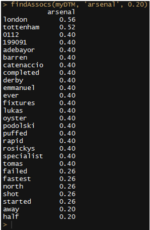
So, London is understandably one of the most commonly used words along with Arsenal, nice to see Rosicky finally start getting some recognition from other football fans, I choose to ignore the fact that Adebayor was placed higher up, he joins my father’s “gaddar” list of Arsenal players (accompanied by RvP, Nasri, Clichy, Cole to name a few.)

But, in the list, oyster seems a little off. I know Arsenal are in London, and London transport is made easier using prepaid cards called Oyster cards, that is a potential outlier, and could involve some investigation later on as to why Joe was tweeting about oyster and Arsenal so often. See, more than halfway in and you’re already picking up patterns that you wouldn’t normally associate with a football club, amazing, that’s data mining for you.

Now, although our documenttermmatrix looks like a matrix, we can’t really process this. We can’t traverse through it by providing a row number and column number to get to a particular entry.

That could be a problem. If only there was a way to convert this into a fully operational matrix with all the features and calculations a matrix offers.

m <- as.matrix(myDTM)

Yeah, it’s that simple. And that’s the beauty of R. You can literally convert from one structure to another with just a single command.

Now that we have our matrix, let me find out the number of occurrences of each term, by adding all the entries for a particular row. At the same time, why not speed things up and sort them in descending order of the count as well?

v <- sort (rowSums(m), decreasing=TRUE)

That creates a handy list of all terms, and their frequency count, in descending order. Let’s create a list of just the names without the numbers then:

 mynames <- names(v)
d<- data.frame(word=mynames, freq=v)

Just converting it to a custom dataframe with the first column named word having the values of mynames, and the second being named freq having the frequency count of each.

Ok, we now have the most common words our good friend Joe has been talking about in the recent past. Let’s make it look pretty, shall we?

wordcloud(d$word, d$freq, min.freq=3)

Create a word cloud, using the variable word and the frequency from the data frame d, and only consider those who have a frequency value of greater than or equal to 3.

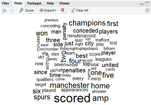
And there we go…. a pretty word cloud that proves one of my long term hunches. Our good friend Joe, is a closet Manchester United fan. Can’t say I’m impressed Joe.

So, twitter data, mined just like that. Not too hard was it?

You could modify the code in so many ways to suit you. If you think about it, just searching for a user’s tweets aren’t that helpful. It’s only giving me information about one user.

Mining according to hashtags is much more informative. It gives me a more diverse public opinion, especially, say if a big event is taking place that has a dedicated twitter hashtag!

We’ll have to modify our code a little bit to take this into consideration. But don’t worry, it’s just the matter of changing one line.

Remember the point where we actually access the twitter database by specifying optajoe’s name?

Well, we just need to modify that one line of code.

rdmTweets2 <- searchTwitter(“ENTER YOUR SEARCH TERM HERE”, n=50)

That’s it. Don’t forget to include the # within the search criteria. So, to know all the details about this weeks #ff, all I need to do is

rdmTweets2 <- searchTwitter(“#ff”, n=50)

Where n specifies the number of tweets we want. This bit of code takes a little bit longer to execute, so don’t be worried that the “>” symbol isn’t showing up on the console(which means that R is waiting for your next command to run) or that there’s suddenly a red circle in the top right border of the console. That happens when R is running a particularly lengthy or complicated bit of code. Just wait till the red dot goes or the > magically reappears.

There’s also so much more you can do. If you notice, once you convert the rdmtweets  into a dataframe (the df<- ) bit, in the top right box of RStudio there is a panel that shows “Environment” and “History”. In Environment, there’s a list of all the variables that you’ve used, and their value, just to keep track. In the data bit, right on top, you’ll find your variable df, and clicking on it should open a table which shows all the values present. We can see the text, the creation date and time of when that tweet was posted, the source of the tweet (android app, web browser, iPhone. The number of times that was retweeted, etc etc. Such a truckload of information which allows you to create all sorts of trends.

And all this data, so easily available. Scary, but also exciting!

Feel free to play around, explore and discover. Maybe next time you’re organising that big event, you can figure out who is tweeting about it and how many times that has been retweeted. Or maybe you’re planning on developing a crude market survey for your product? Or maybe you’re just curious about how many times Ellen’s famous record-breaking Oscar selfie was actually retweeted (3405717 as of when I last checked. ). It takes just 30 seconds (once you’ve set up R and your Twitter OAuth.)

That’s it. I hope the code was easy enough to follow, I’ve tried my best to explain in very simple terms, but I’ve been around coding and computers since I was 10 and used to draw triangles using LOGO (right 90, left 180) and maybe something that’s befuddling to you totally skipped my mind. Do let me know, I want this post to hopefully help everyone realise how awesome coding can be, and how it’s really not as hard as it’s made out to be.
As promised, the code in entirety can be found here:

install.packages(“twitteR”)
install.packages(“tm”)
install.packages(“SnowballC”)
install.packages(“wordcloud”)

library(twitteR)
library (RCurl)
library(tm)
library(SnowballC)
library(wordcloud)

download.file(url=”http://curl.haxx.se/ca/cacert.pem&#8221;, destfile=”cacert.pem”)

options(RCurlOptions = list(cainfo = system.file(“CurlSSL”, “cacert.pem”, package = “RCurl”)))

reqURL <- “https://api.twitter.com/oauth/request_token&#8221;
accessURL <- “https://api.twitter.com/oauth/access_token&#8221;
authURL <- “https://api.twitter.com/oauth/authorize&#8221;
apiKey <- “INSERT API KEY HERE”
apiSecret <- “INSERT API SECRET HERE”

twitCred <- OAuthFactory$new(consumerKey=apiKey,consumerSecret=apiSecret,requestURL=reqURL,accessURL=accessURL,authURL=authURL)

twitCred$handshake(cainfo = system.file(“CurlSSL”, “cacert.pem”, package = “RCurl”))

registerTwitterOAuth(twitCred)

rdmTweets2 <- userTimeline(“optajoe”, n=200)
n<- length(rdmTweets2)

df <- do.call(“rbind”, lapply(rdmTweets2, as.data.frame))
dim(df)

mycorpus<- Corpus(VectorSource(df$text))
mycorpus <- tm_map(mycorpus, tolower)
mycorpus <- tm_map(mycorpus, removePunctuation)
myStopWords <- c(stopwords(“english”), “english”, “premier”, “league”, “epl”, “football”)
mycorpus <- tm_map(mycorpus, removeWords, myStopWords)

#inspect(mycorpus[1:3])

myDTM <- TermDocumentMatrix(mycorpus, control=list(minWordLength=1))
findAssocs(myDTM, ‘arsenal’, 0.20)
m <- as.matrix(myDTM)
v <- sort (rowSums(m), decreasing=TRUE)

mynames <- names(v)
d<- data.frame(word=mynames, freq=v)

wordcloud(d$word, d$freq, min.freq=3)